Introduction
Metabolic diseases afflict millions of people in the US, with diseases such as diabetes, high blood pressure, and obesity affecting Latinos and other ethnic minority groups at a significantly higher rate. Our project seeks to further metabolic disease research and expand representation in such fields by studying how the gut microbiomes of Hispanic populations are correlated with the prevalence of certain diseases. The main goal of our project is to use the Study of Latinos (SOL) gut microbiome dataset to implement and train machine learning models that can determine an individual’s metabolic disorders based on their gut microbiome. To achieve our goal, we will utilize a binary-relevance model for each disease type to see if we can predict the appearance of a disease in an individual according to their microbiome factors.
Data Description
The SOL is a population-based study of Hispanic/Latino adults from the ages of 18-74 who were selected from randomly sampled census block areas in the US. For our project, we will be using 1835 self-collected stool samples that is broken into two main parts, (1) the frequency table of genomic sequences and (2) the metadata. The dataset is available on Qiita (https://qiita.ucsd.edu/) ID: 11666.
(1) A genomic sequence is the information given by an organism’s DNA/RNA, each column in our frequency table corresponds to an organism’s genomic sequence (in our case some sort of bacteria in our gut). The frequency table of genomic sequences counts the number of times that a unique genomic sequence appears in a sample.
(2) The metadata, among other things, contains information about whether the participants had a certain metabolic disease. A subset of the diseases will be selected as our classification targets and a few metadata columns such as age and gender will be used as features in addition to the entire feature table of genome sequences.
Exploratory Data Analysis
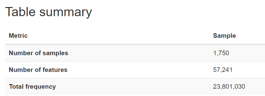
After dropping the samples with missing values and identifying the samples that existed in both the feature table and metadata, we found 1750 samples that we could use for our analysis.
Metadata Analysis
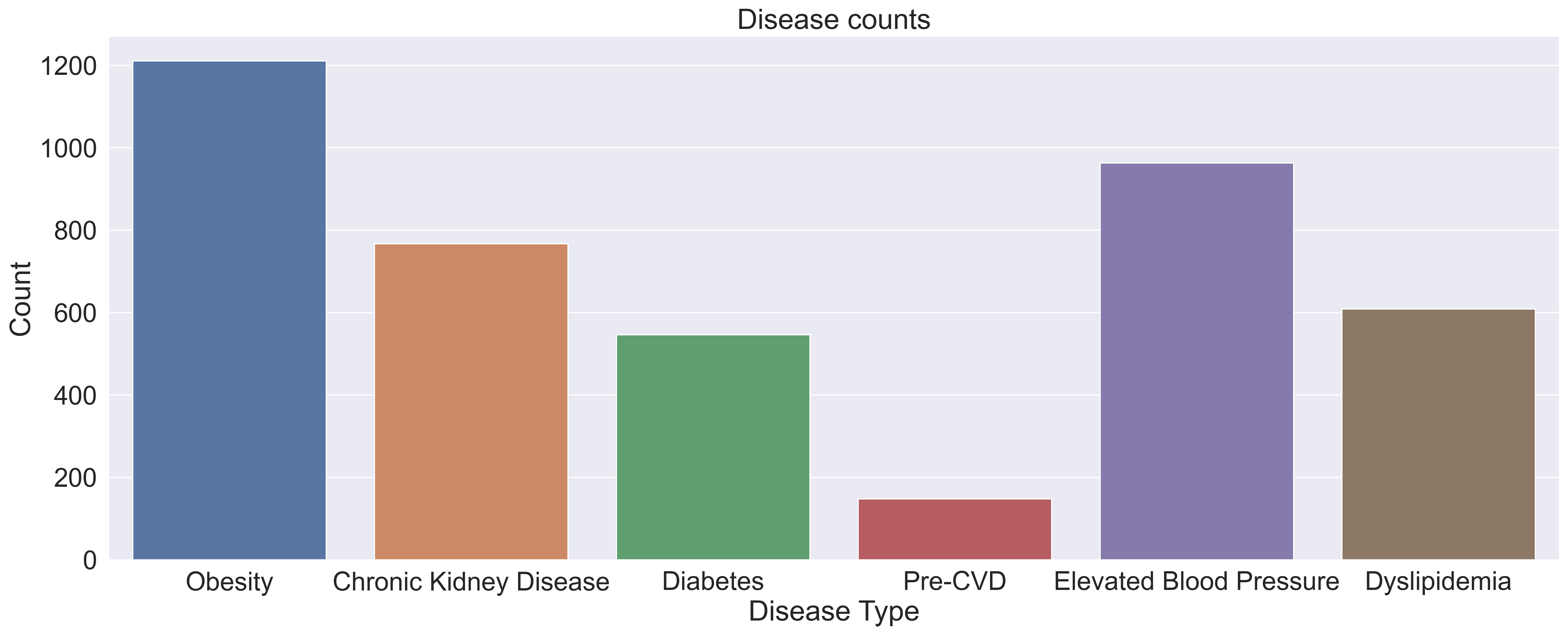
Within the 1750 samples, we can see in the graph below, pre-cvd had by far the lowest presence within our dataset, indicating that there might be a large class imbalance within the pre-cvd colum. This class imbalance will need to be addressed in our pre-processing in order to prevent our model from overfitting.
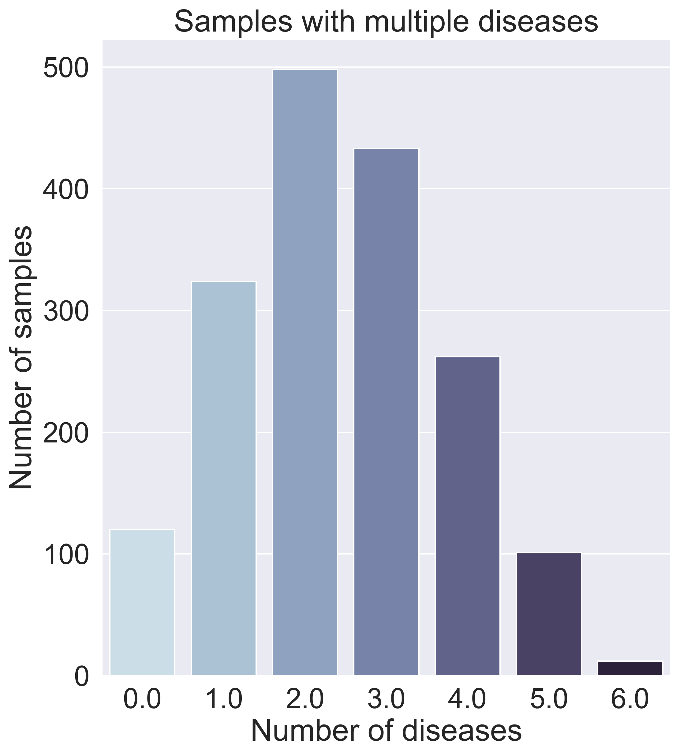
After further data exploration, we found that many samples have varying amounts and varying combinations of diseases, as can be seen in the graph below, which means a binary classifier (predicting what disease someone has) would not work.
Dimensionality Analysis
The nature of microbiome data is that it is extremely high in dimensions. Our frequency table had over 57,000 columns/features with over 23 million reads for the 1750 participants. With such high dimensions it is hard to extract any patterns in the data, therefore dimensionality reduction of the features (columns) is required.
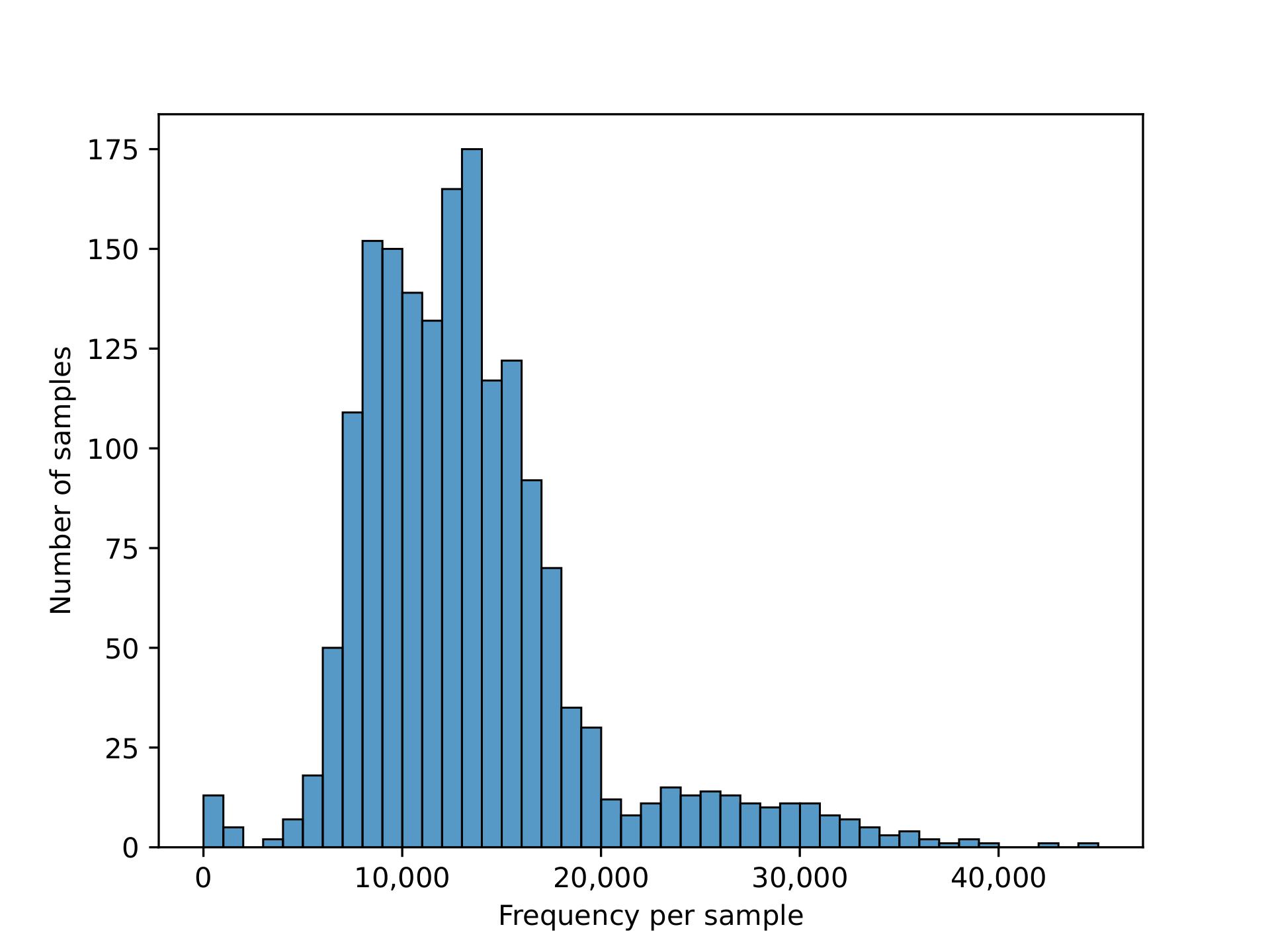
We plotted the count/frequency of samples that each feature appears on in our feature table dataset. By looking at this plot we see that alot of our features have very low sample frequencies, which means that theres a lot of irrelevant features/columns that have little importance and could be dropped in our data.
After setting a feature importance threshold method, we reduced the number of features to around 4000 from the 57,000 we had before
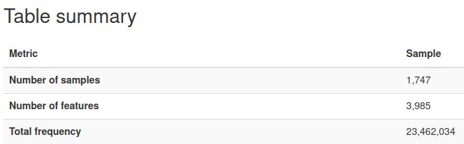
We also were able to increase the mean frequency per feature from around 400 to 5000 per feature (higher mean frequency means less noise, and features encompass more information)
PcOA and UMAP
Principal Coordinate Analysis (PCoA) and Uniform Manifold Approximation & Projection (UMAP) are the 2 dimension reduction techniques we used to help us further understand the frequency table. We planned on using the reduced dimension data to visualize any patterns/clustering in our data and use the dimension-reduced embeddings as features for our classification model.
For our first attempt at visualizations, we plotted PCoA plots in the 3D space using a variety of distance metrics for comparison, but found that clustering is difficult to see. We believe this is caused because of varying amounts and varying combinations of diseases that individuals/samples have, as previously mentioned in our metadata analysis.
3D Plots of PCoA comparisons for Diabetes
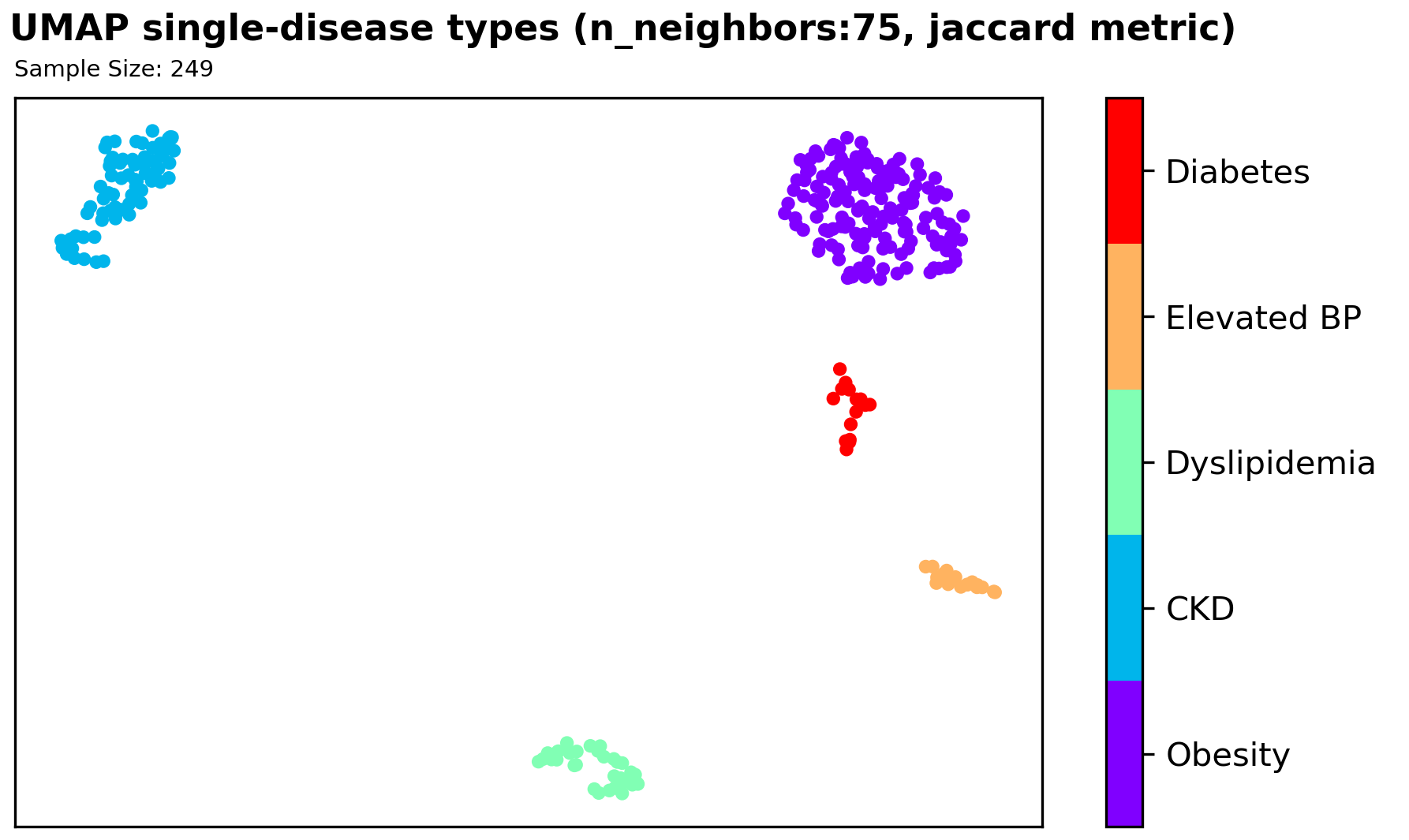
We found significant clustering results with a supervised UMAP in the 2D space using a Jaccard distance metric, which signifies that further exploration of using this method could be useful for our classification problem. However, since we have very limited sample size, and an imbalanced disease types among samples, it is hard to utilize our finding as information/features for our classification model.
Machine Learning Models
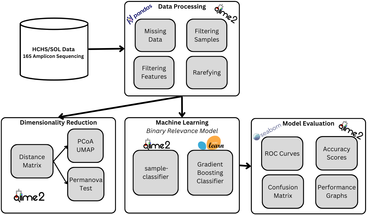
Because our task involves determining which specific diseases a sample has, we took a multi-label approach to building our machine learning model. A basic binary relevance model was implemented as a baseline model. An independent binary classifier was created, trained, and tuned for each class (disease), and each sample is then inputted into each classifier to see if that sample has that particular disease or not.

While this binary relevance model is quick to implement and train, it assumes independence between all of our classes, which is likely not true in our case. Studies have shown diseases like obesity and diabetes are correlated, so finding a model that can account for such relations would help the accuracy and scalability of our model to more and other diseases.
Results
Statistical Tests with PERMANOVA
The table below demonstrates the p-values of the PERMANOVA tests computed for each disease type using unweighted and weighted UniFrac distance matrices.
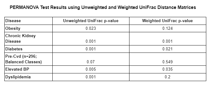
As we can see in the table above, the majority of PERMANOVA tests computed had a p-value less than 0.05 which means that the null hypothesis is rejected in those cases. This means that the observed differences between those who had a given disease and those who did not, is likely not due to chance alone and indicates that another factor/variable is leading to the differences between both groups (those with and those without a given disease). The only PERMANOVA tests that had a p-value higher than .05 were both pre-cvd tests and the obesity test using the weighted UniFrac distance matrix. We suspect that pre-cvd tests were likely affected by the class balancing, which resulted in a loss of information.
Model Accuracies
The plot below shows the performance of each individual gradient boosting binary classification model within our binary relevance model. The plot contains the overall accuracy, the macro-average, and micro-average area under the curve (AUC’s) for the model’s receiver operating characteristic (ROC) curves.
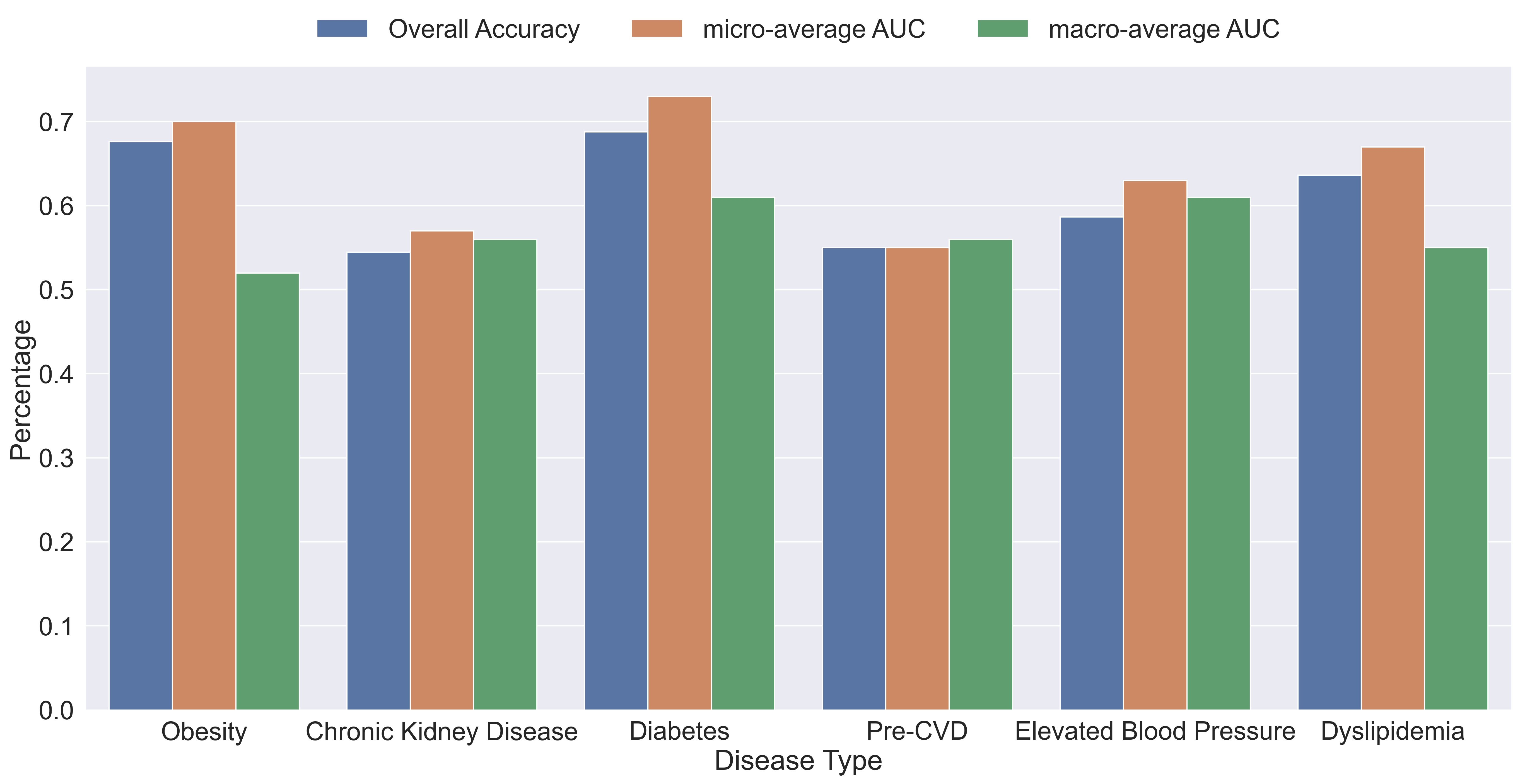
As we can see by the results, the average overall accuracy of the models was about 60.9% and all the AUC’s are above 50% which means that every model performed better than random chance. Obesity and diabetes were the best performing models with an accuracy of about 67% and 69%, micro-average of about 70% and 73%, and macro-average of about 51% and 61%, respectively. The big difference between micro and macro-average AUC’s of the obesity model indicates that the model performs better on the majority class than on the minority class, which indicates that we may need to do more pre-processing to improve the results.
It’s possible that different choices of classifiers or models could be implemented to improve our task performance. As seen in the PERMANOVA test, there are significant and obvious differences between the metabolic diseases when looking at samples with only one disease. However, because the majority of our samples have multiple diseases, it is reasonable to assume the microbiome features would look very differently, requiring models or special inputs that recognize the how having multiple diseases can impact the features and vice versa.
Conclusion
Overall, due to the difficulty of multi-label classification tasks, the high count of disease co-occurence, the complexity of microbiome and disease research, and the lack of substantial/balanced data, the results yielded by our model has a lot of room for improvement. The low accuracy of our model suggests a different multi-label machine learning model or further data pre-processing may be required.
Even though our project did not yield our desired results, our project still contributes to the field of gut microbiome research by performing analysis with Python and commonly used Python packages, lowering the barrier of entry for other data scientists and equipping current researchers with new tools such as qiime2.